Exercise #4 -- Analysis and Visualization

AIDA is still fairly new so currently there is some variation between the completeness of the various implementations, but a comprehensive test suite has just been completed which will allow implementations to be checked for compatibility in future.

By developing examples and tutorials based on the AIDA interfaces Geant4 is able to work with any AIDA compliant analysis system. In this workshop we will concentrate on using the JAIDA implementation with AIDAJNI, because of its cross-platform nature and our local expertise. However the techniques used should work with other AIDA implementations.

More information on AIDA is available from:

• The AIDA home page
• The AIDA Users Guide (unfortunately the examples here are all in Java, but the translation to C++ is straightforward, and coupled with the example code provided as part of the A01 tutorial should be quite understandable). C++ examples will be added in the near future.

Turning on Analysis in example A01

The A01 example used in this workshop has been set up to use AIDA for analysis. The example shows how to create histogram and tuples, how to save these to a file, and how to view plots interactively.

To turn the visualization in example A01 on you must first install an implementation of AIDA. This CD contains JAIDA, a Java implementation of AIDA, and AIDAJNI, an AIDA bridge to allow communication between C++ and Java.

If you do not have JAVA 1.4.1 or later installed you must first install it. Java is available on this CD. Once you have installed Java you must set an environment variable JDK_HOME to point to the location where you installed it, e.g.

export JDK_HOME=c:/j2sdk1.4.2

Now unpack the appropriate versions of AIDAJNI and JAIDA, and then set the environment variables JAIDA_HOME and AIDAJNI_HOME to point to the location where you unpacked the files, and then source the appropriate setup script e.g.:

Windows:

export JAIDA_HOME=c:/JAIDA-3.2.0
source $JAIDA_HOME/bin/aida-setup.win32

export AIDAJNI_HOME=c:/AIDAJNI-3.0.4
source $AIDAJNI_HOME/bin/WIN32-VC/aidajni-setup.win32

Unix sh:

export JAIDA_HOME=`pwd`/JAIDA-3.2.0
source $JAIDA_HOME/bin/aida-setup.csh

export AIDAJNI_HOME=`pwd`/AIDAJNI-3.0.4
source $AIDAJNI_HOME/bin/Linux-g++3/aidajni-setup.csh

Unix csh:

setenv JAIDA_HOME `pwd`/JAIDA-3.2.0
source $JAIDA_HOME/bin/aida-setup.csh

setenv AIDAJNI_HOME `pwd`/AIDAJNI-3.0.4
source $AIDAJNI_HOME/bin/Linux-g++3/aidajni-setup.csh

(The setup scripts are available with several prefixes: win32 for cygwin,. csh for unix c-shell, .sh for unix shell/bash -- make sure you use the appropriate version).

Now to turn on analysis in the A01 example you must set the environment variable G4ANALYSIS_USE and rebuild the example. Note: If you have previously turned on OpenGL you must turn it off, since currently you cannot have OpenGL and JAIDA enabled at the same time:

export G4ANALYSIS_USE=1
export G4VIS_USE_OPENGLX=
export G4VIS_USE_OPENGLXM=
make clean
make

You can now run the A01 example again:

$G4INSTALL/bin/$G4SYSTEM/A01app
Idle> /run/beamOn 100

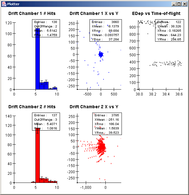
This time as your analysis runs a window should appear showing the histograms being filled. The window should look something like this.

When you exit the example it will also create an A01.aida file, which contains the final histograms and n-tuples. This file can be analyzed by any AIDA compliant analysis tool, such as JAS3 (see instructions below)

Creating Your Own Histograms

Two classes in the A01 example do all the analysis work. These are:

• A01AnalysisManager - This class is a simple wrapper around the AIDA factories used to create Histograms, Plotters and Tuples. You should not need to modify this class, but you may want to take a look at it to understand what it is doing. The useful methods it defines are:
  • static T01AnalysisManager* getInstance() - Get the (singleton) instance of T01AnalysisManager
  •  IHistogramFactory* getHistogramFactory() - Used for creating histograms and clouds (unbinned histograms)
  • ITupleFactory* getTupleFactory() - Used for create tuples
  • IPlotter* createPlotter() - Create a Plotter (used for displaying histograms and clouds)
• A01EventAction - This is where the user defined analysis is performed. After reading the AIDA Users Guide the code here should be fairly self explanatory.

A good exercise would be to add you own histograms and display them using the plotter, or add your own columns to the Tuple.

Using JAS3 to Analyze .aida Files

When you ran the A01 example earlier it should have created a file A01.aida. (This file is also available on the CD here). You can open this file with any AIDA compliant tool. One such tool, JAS3, is included on this CD, or can be downloaded from http://jas.freehep.org/jas3. Installing JAS3 should be quite straightforward, installation instructions are available as part of the JAS3 tutorial.

Once you have installed and stared JAS you can open the A01.aida file using the File, Open File menu item

.

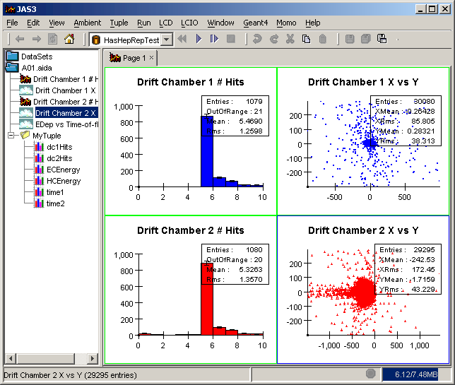
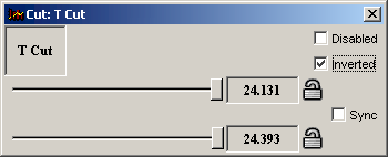
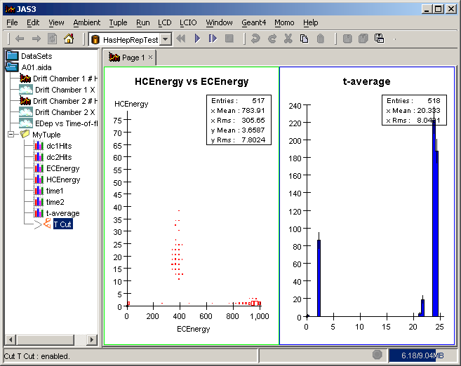
You can now view the histograms and clouds by either:

• Double-clicking their icon's in the tree below the A01.aida node
• Right clicking on their icon's and selecting items from the popup menu
• Dragging icons from the tree onto the plot page. You can create new plot pages using File, New, Plot Page, and can change the properties of the plots and the plot page by right clicking on the page.

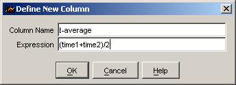
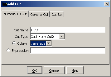
You can also explore columns on the n-tuple produced by Geant4. You can:

• Double-click on columns to plot them
• Right click on columns and select different options. You can also click on multiple columns to make 2d plots, or to tabulate selected columns.
• Click on the "My Tuple" node to create cuts, define new columns etc.

Example are shown below:

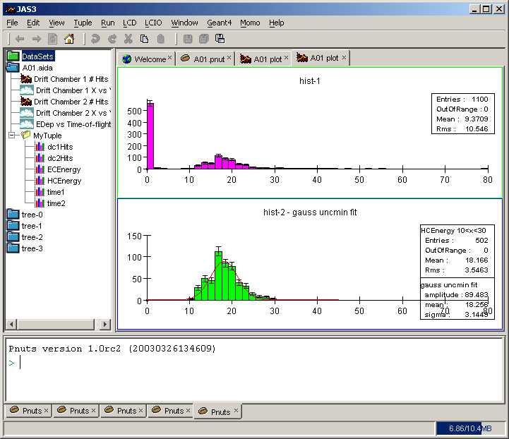
In addition to using the JAS3 GUI directly you can also script JAS3 in Python, Pnuts or Java. To do so you use precisely the same AIDA interfaces that you used inside Geant4. Here is a sample Pnuts script which shows how to access the HCEnergy column from the MyTuple tuple, apply a cut, project into a histogram, fit the result with a Gaussian, and plot the result.

IAnalysisFactory = class hep.aida.IAnalysisFactory
af = IAnalysisFactory::create()
tree = af.createTreeFactory().create()
tf = af.createTupleFactory(tree)
hf = af.createHistogramFactory(tree)

// Locate the tuple

tuple = aidaMasterTree.find("A01.aida/MyTuple");

// make a plot of the HCEnergy

energy = tf.createEvaluator("HCEnergy")
h1 = hf.createHistogram1D("hist-1", "HCEnergy", 50, 0, 80)
tuple.project(h1, energy)

// Make a plot of HCEnergy with a cut

h2 = hf.createHistogram1D("hist-2", "HCEnergy 10<x<30", 50, 0, 80)
cut = tf.createFilter("HCEnergy>10 && HCEnergy<30");
tuple.project(h2, energy, cut)

// Perform a simple fit

ff = af.createFunctionFactory(tree)
gauss = ff.createFunctionByName("gauss","g")
gauss.setParameter("amplitude",h2.maxBinHeight())
gauss.setParameter("mean",h2.mean())
gauss.setParameter("sigma",h2.rms())

fitter = af.createFitFactory().createFitter("Chi2")
result = fitter.fit(h2,gauss)

// Plot the results

plotter = af.createPlotterFactory().create("A01 plot");
plotter.createRegions(1,2,0);
plotter.region(0).plot(h1);
plotter.region(1).plot(h2);
plotter.region(1).plot(result.fittedFunction());
plotter.show();

You can run the script by selecting File, New, Pnuts Script, pasting the code above into the resulting editor window, and then clicking F2 (=Run). Here is the result:

We have only been able to give a brief taste of using AIDA/JAS3 here. For more information on using JAS3 for Geant4 and beyond see the JAS3 Tutorial.