[Feedback][Day 1][Day 2][Welcome Page]

Fast Monte Carlo Example

If you have worked through the previous tutorials in this series, then you should know how to open a stdhep file and compile and load the analysis routine provided below. The example makes use of the ability of a Driver to have one or more Processors added to it. By default the process method of Driver will call each of the Processors in turn. In this example we add two Processors to our main Driver, MCFast, which is a Processor provided with the LCD extensions, and ResCheck, which is a user supplied processor where we do some histogramming on the output of the FastMC.

Note that since we are reading generator level data we have to explicitly tell the lcd software which detector geometry to use. The statements

      String detector = "sdmar01";
      Detector.setCurrentDetector(new Detector(detector));

do that. (We could also have used ldmar01 as the detector name).

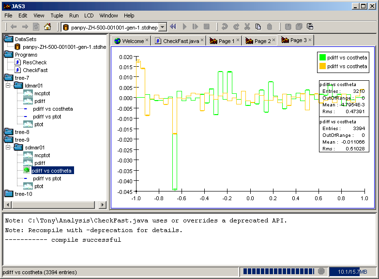
The ResCheck class is also defined in the example. It extends AbstractProcessor and overrides the process method as we did in the previous example. The example also shows how to use profile plots in AIDA/JAS3.

import hep.physics.*;
import hep.lcd.event.*;
import hep.lcd.mc.fast.*;
import hep.lcd.util.driver.*;
import hep.lcd.geometry.*;
import java.util.*;

final public class CheckFast extends Driver
{
   public CheckFast() throws java.io.IOException
   {
      String detector = "sdmar01";
      Detector.setCurrentDetector(new Detector(detector));
      tree().mkdirs("/"+detector);
      add(new MCFast());
      add(new ResCheck(detector)); // user analysis routine
   }
}
class ResCheck extends AbstractProcessor
{
   private String folder;
   ResCheck(String folder)
   {
     // create some special histograms
     this.folder = folder;
   }
   public void process(LCDEvent event)
   {
     tree().cd("/"+folder);
     // Loop over tracks
     Enumeration e = event.getTrackList().getTracks();
     while (e.hasMoreElements())
     {
        Track t = (Track) e.nextElement();
        double ptot = Math.sqrt(t.getMomentumX()*t.getMomentumX() +
                                t.getMomentumY()*t.getMomentumY() +
                                t.getMomentumZ()*t.getMomentumZ());
        // Get associated MC particle
        MCParticle mc = t.getMCParticle();
        double mcptot = Math.sqrt(mc.getPX()*mc.getPX() +
                                  mc.getPY()*mc.getPY() +
                                  mc.getPZ()*mc.getPZ());
        double cosTheta = mc.getPZ()/mcptot;
        double pdiff = mcptot - ptot;
        
        // Make some plots
        cloud1D("pdiff").fill(pdiff);
        cloud1D("ptot").fill(ptot);
        cloud1D("mcptot").fill(mcptot);
        profile1D("pdiff vs ptot",50,0,50).fill(ptot,pdiff);
        profile1D("pdiff vs costheta",50,-1,1).fill(cosTheta,pdiff);
      }
   }
}

Comparing the Different Detector Responses

The ResCheck class in the above example puts all of the created histograms into a folder named after the detector used. This makes is possible to run the routine more than once on the same input data to compare the responses of the two detectors. You would do this as follows:

Compile and load the program as written, and the run through all of the data (using Job, Go).
Now modify the routine so that detector is set to ldmar01 instead of sdmar01, and recompile. (The recompiled routine will automatically replace the already loaded routine).
To run through the data again you must first rewind the data (using Job, Rewind), but by default JAS will clear all the histograms when you rewind, so you must first select the Histograms/sdmar01 folder in the tree on the left of the JAS window, right click, and from the popup menu turn off Clear On Rewind.
Now rewind and run through the data again, and you will have two folders, one containing the SD results and one containing the LD results. You can overlay histograms by double-clicking one, and then right clicking on the corresponding histogram from the other folder and selecting Overlay.

Using WIRED with the FastMC

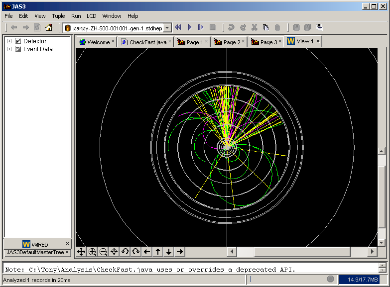
The WIRED event display described in the earlier tutorial with work with the results of the FastMC. You can use it to compare the MC truth tracks with the Fast MC output.

Go to the next tutorial.